2D plotting functionalities for POSYDON GRIDS

Similar to our 1D plotting functions, we provide a series of 2D plotting functionalities within POSYDON. The plot2D method supports either a MESA grid which samples the 2D parameter space of binary initial conditions or a 4D or 3D MESA grid sampling, e.g., star_1_mass, star_2_mass, period_days, metallicity. In the latter case the grid will be sliced along two dimensions specified by the user.

We illustrate some of the plotting capabilities of plot2D by loading the HMS-HMS grid and reproduce some figures included in the POSYDON instrument paper.

# to load a grid
from posydon.grids.psygrid import PSyGrid
grid = PSyGrid("/PATH_TO_POSYDON_DATA/HMS-HMS/grid_0.0142_%d.h5")

How to plot the MESA termination flags

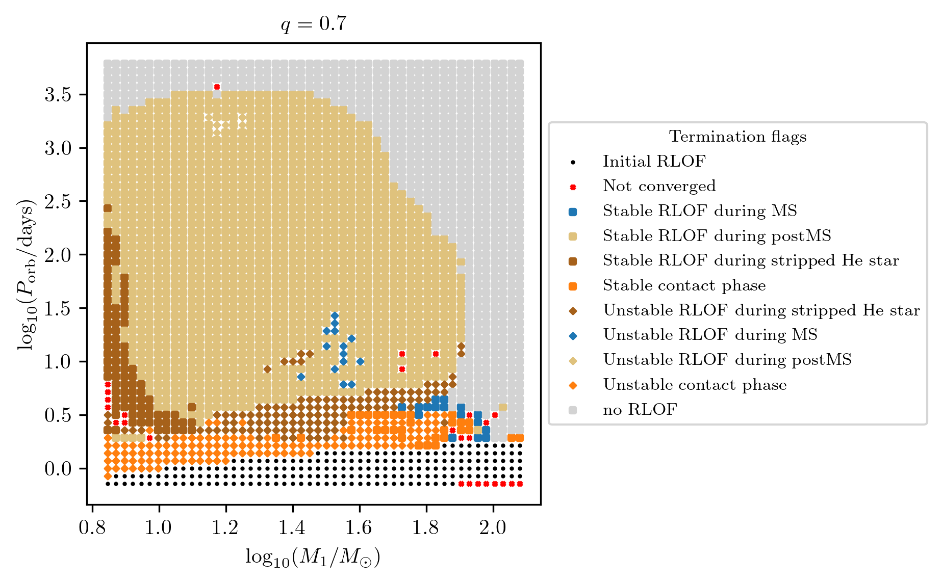
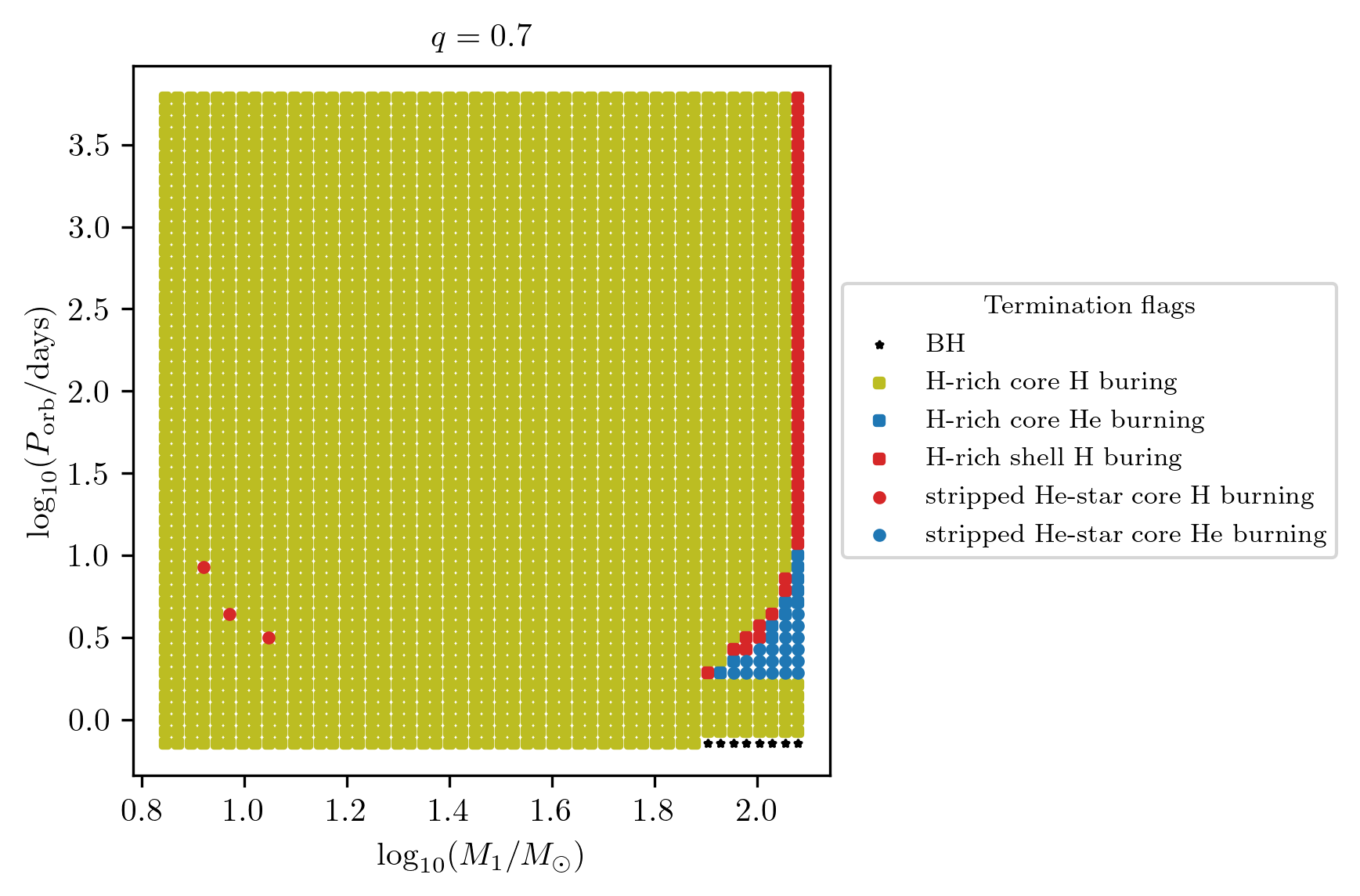
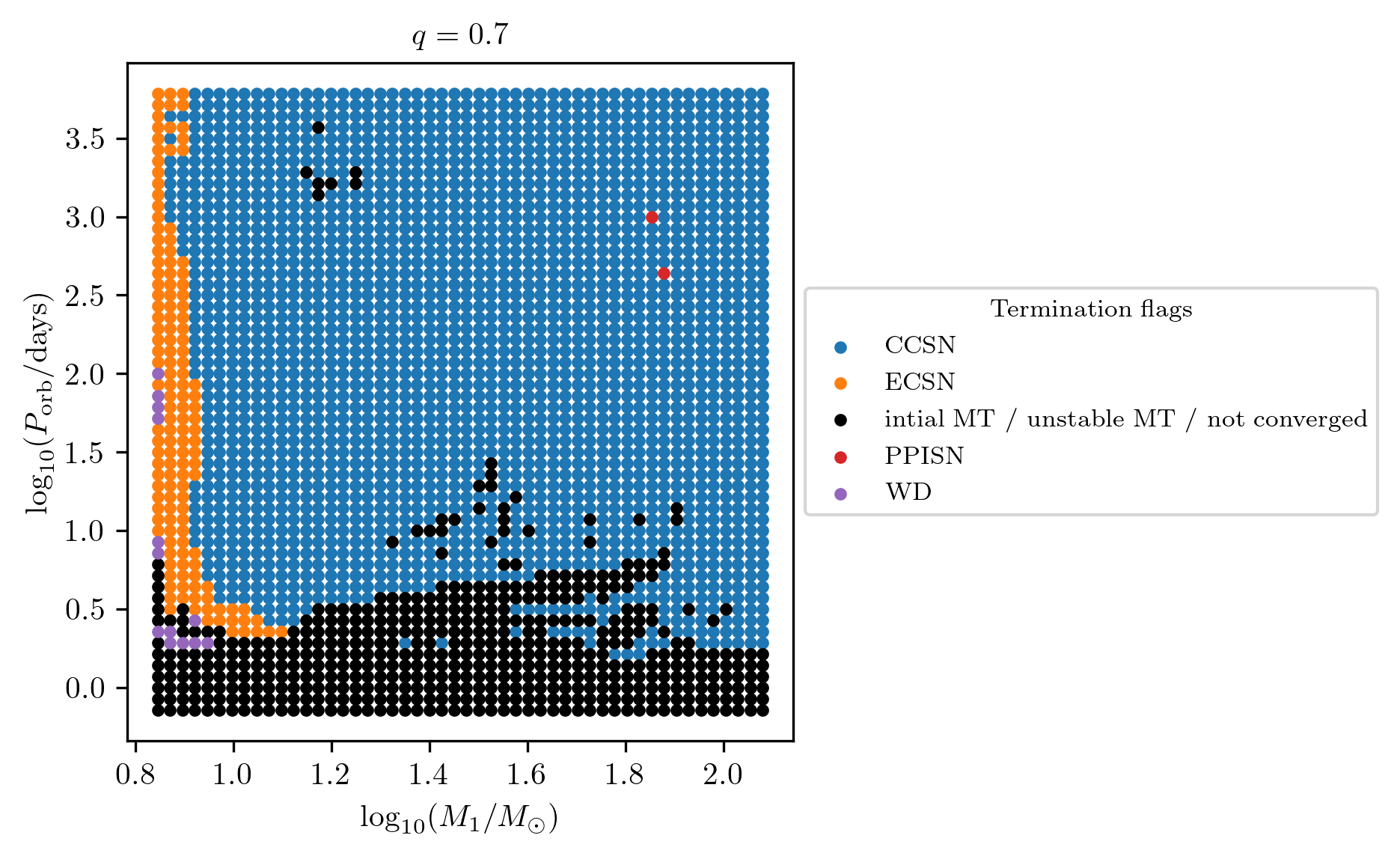
Termination flag 1 & 2 combined

Any plotting parameter is passed to the plot2D method through the kwarg PLOT_PROPERTIES. In our case we would like to visualize the figure, save it to a given path_to_file with filename fname and then close it. Recall that the HMS-HMS grid sampled the initial binary parameter space in star_1_mass, period_days and mass_ratio. To reproduce Fragos et al. (2022) Figure 1, we will slice the 3D parameter space along the mass ratio at q=0.7. We will also set the x and y axis to be displayed in log-space and reduce the default marker size with the following code

q = 0.7
PLOT_PROPERTIES_TF12 = {
    'figsize': (4.5, 4.),
    'show_fig' : True,
    'close_fig' : True,
    'path_to_file': './plots_demo/',
    'fname': 'q_%1.1f_TF12.png'%q,
    'title' : r'$q = %1.1f$'%q,
    'log10_x' : True,
    'log10_y' : True,
}

fig = grid.plot2D('star_1_mass', 'period_days', None,
             termination_flag='combined_TF12',
             grid_3D=True, slice_3D_var_str='mass_ratio',
             slice_3D_var_range=(q-0.025,q+0.025),
             verbose=False, **PLOT_PROPERTIES_TF12)

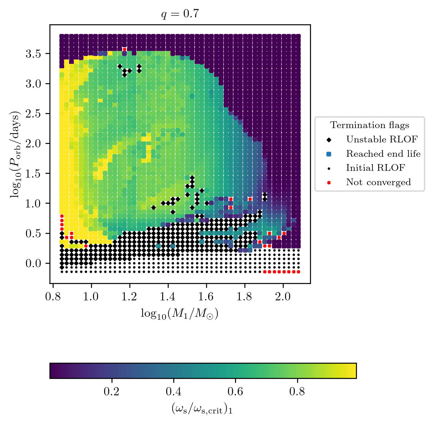
Termination flag 1

Similarly we can plot the termination flag 1 which indicates how the MESA simulation ended. We can display as a color map any final value stored in final_values. This code shows how to reproduce Fig. 10 of Fragos et al. (2022).

PLOT_PROPERTIES_TF1 = PLOT_PROPERTIES_TF12
PLOT_PROPERTIES_TF1['fname'] = 'q_%1.1f_TF1.png'%q
PLOT_PROPERTIES_TF1['figsize'] = (4.5,6.)

fig = grid.plot2D('star_1_mass', 'period_days', 'S2_surf_avg_omega_div_omega_crit',
             termination_flag='termination_flag_1',
             grid_3D=True, slice_3D_var_str='mass_ratio',
             slice_3D_var_range=(q-0.025,q+0.025),
             verbose=False, **PLOT_PROPERTIES_TF1)

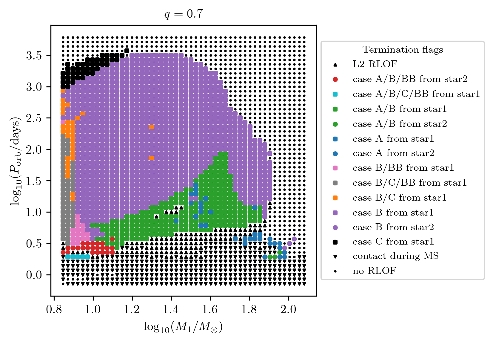
Termination flag 2

The termination flag 2 shows a summary of all mass transfer cases which occurred during the binaries’ evolution.

PLOT_PROPERTIES_TF2 = PLOT_PROPERTIES_TF12
PLOT_PROPERTIES_TF2['fname'] = 'q_%1.1f_TF2.png'%q

fig = grid.plot2D('star_1_mass', 'period_days', None,
             termination_flag='termination_flag_2',
             grid_3D=True, slice_3D_var_str='mass_ratio',
             slice_3D_var_range=(q-0.025,q+0.025),
             verbose=False, **PLOT_PROPERTIES_TF2)

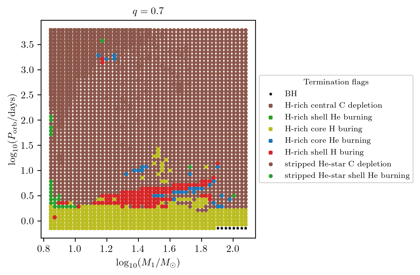
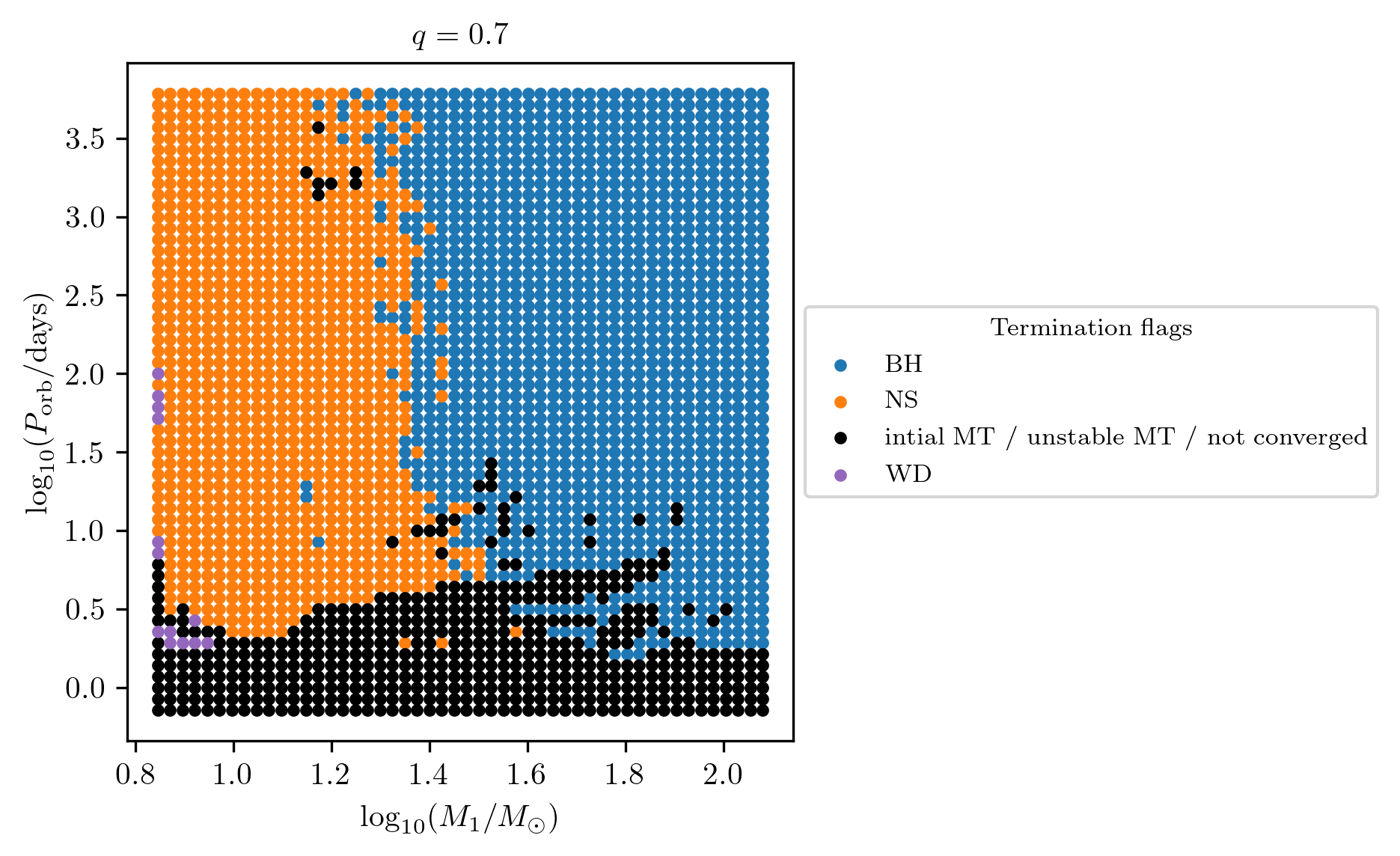
Termination flag 3

The termination flag 3 shows the final stellar state of star 1.

PLOT_PROPERTIES_TF3 = PLOT_PROPERTIES_TF12
PLOT_PROPERTIES_TF3['fname'] = 'q_%1.1f_TF3.png'%q

fig = grid.plot2D('star_1_mass', 'period_days', None,
             termination_flag='termination_flag_3',
             grid_3D=True, slice_3D_var_str='mass_ratio',
             slice_3D_var_range=(q-0.025,q+0.025),
             verbose=False, **PLOT_PROPERTIES_TF3)

Termination flag 4

The termination flag 4 shows the final stellar state of star 2.

PLOT_PROPERTIES_TF4 = PLOT_PROPERTIES_TF12
PLOT_PROPERTIES_TF4['fname'] = 'q_%1.1f_TF4.png'%q

fig = grid.plot2D('star_1_mass', 'period_days', None,
             termination_flag='termination_flag_4',
             grid_3D=True, slice_3D_var_str='mass_ratio',
             slice_3D_var_range=(q-0.025,q+0.025),
             verbose=False, **PLOT_PROPERTIES_TF4)

All termination flags

We plot all termination flags at once in a large subplot of panels with the option termination_flag='all'. In order to fit all legends we suggest to increase the figure size and marker size to, e.g. (25,25) and 30, respectively.

Display custom quantities

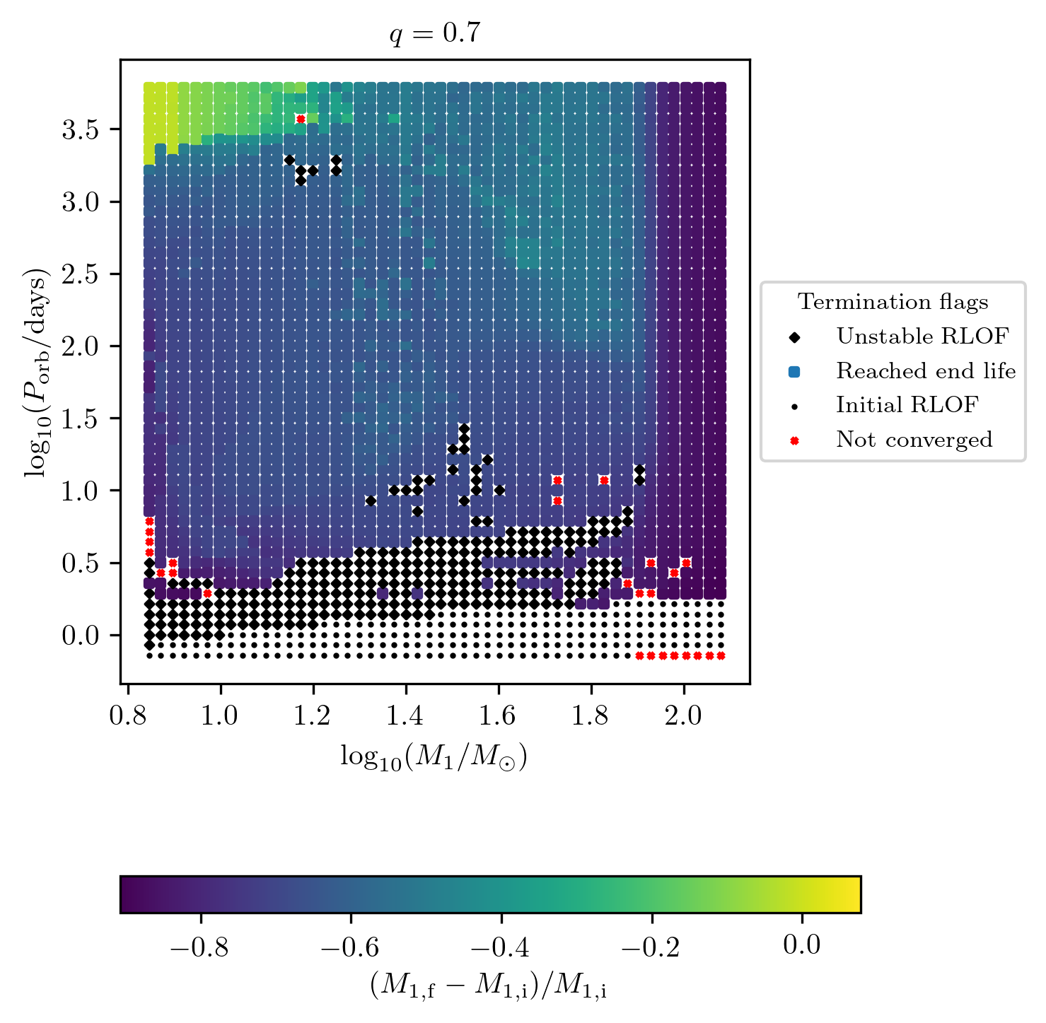
Relative change of a final quantity

The relative change of any value stored within final_values can be displayed by adding the prefix relative_change_ to the z-variable displayed as a colorbar. E.g. we can display the relative change of star_1_mass:

PLOT_PROPERTIES_TF1 = PLOT_PROPERTIES_TF12
PLOT_PROPERTIES_TF1['fname'] = 'q_%1.1f_TF1_DM1.png'%q
PLOT_PROPERTIES_TF1['figsize'] = (4.5,6.)
PLOT_PROPERTIES_TF1['colorbar'] = {'label' : r'$(M_\mathrm{1,f}-M_\mathrm{1,i})/M_\mathrm{1,i}$',}

fig = grid.plot2D('star_1_mass', 'period_days', 'relative_change_star_1_mass',
             termination_flag='termination_flag_1',
             grid_3D=True, slice_3D_var_str='mass_ratio',
             slice_3D_var_range=(q-0.025,q+0.025),
             verbose=False, **PLOT_PROPERTIES_TF1)

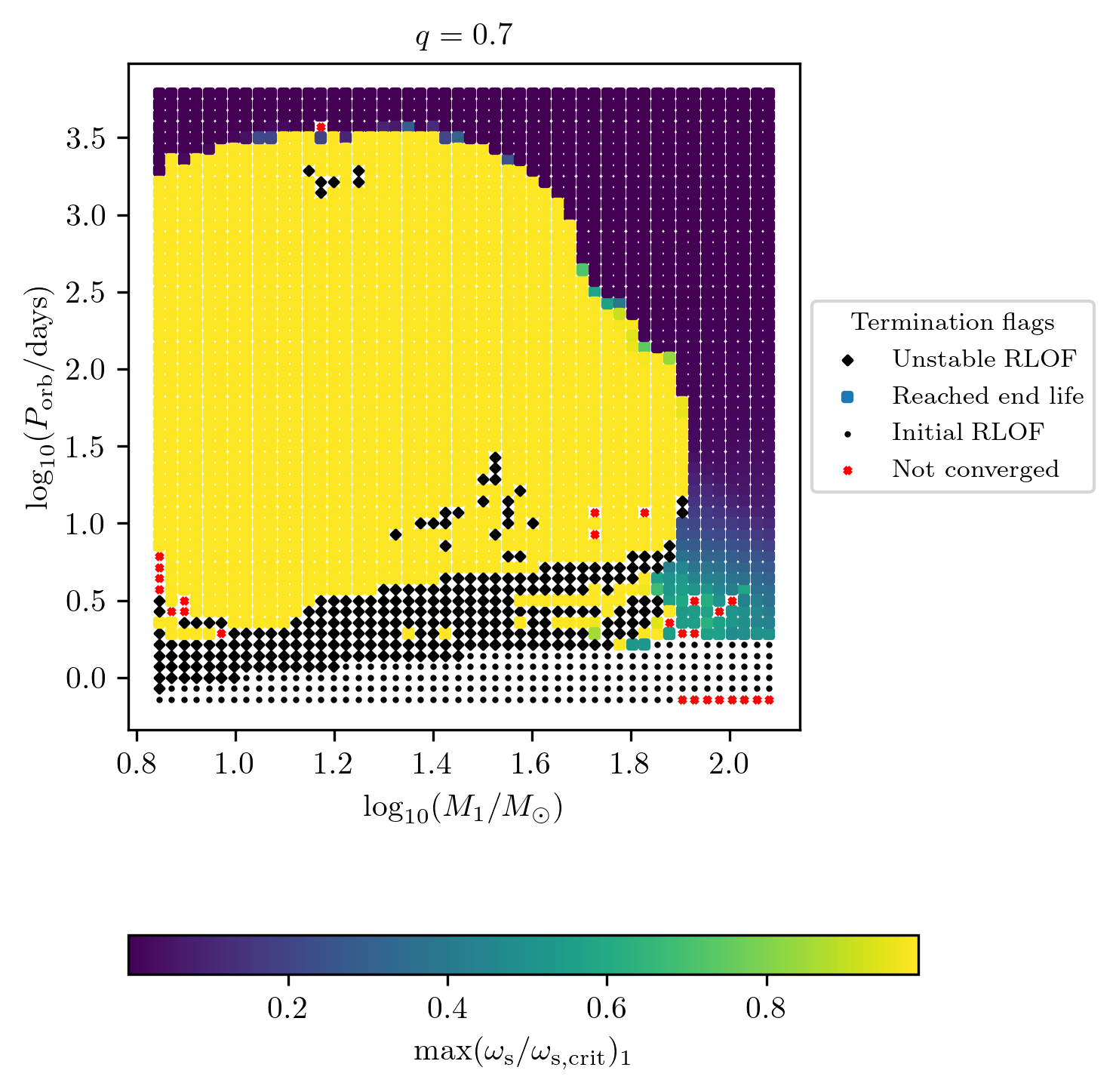
Custom quantities

The user can plot custom quantities as a color map on termination flag 1. For example, we display the maximum surf_avg_omega_div_omega_crit during the history of star 2 as follows

PLOT_PROPERTIES_TF1 = PLOT_PROPERTIES_TF12
PLOT_PROPERTIES_TF1['fname'] = 'q_%1.1f_TF1_max.png'%q
PLOT_PROPERTIES_TF1['figsize'] = (4.5,6.)
PLOT_PROPERTIES_TF1['colorbar'] = {'label' : r'$\max(\omega_\mathrm{s}/\omega_\mathrm{s,crit})_1$'}

max_omega = [max(grid[i].history2['surf_avg_omega_div_omega_crit'])
            if grid[i].history2 is not None else np.nan
            for i in range(len(grid.MESA_dirs))]

fig = grid.plot2D('star_1_mass', 'period_days', np.array(max_omega),
             termination_flag='termination_flag_1',
             grid_3D=True, slice_3D_var_str='mass_ratio',
             slice_3D_var_range=(q-0.025,q+0.025),
             verbose=False, **PLOT_PROPERTIES_TF1)

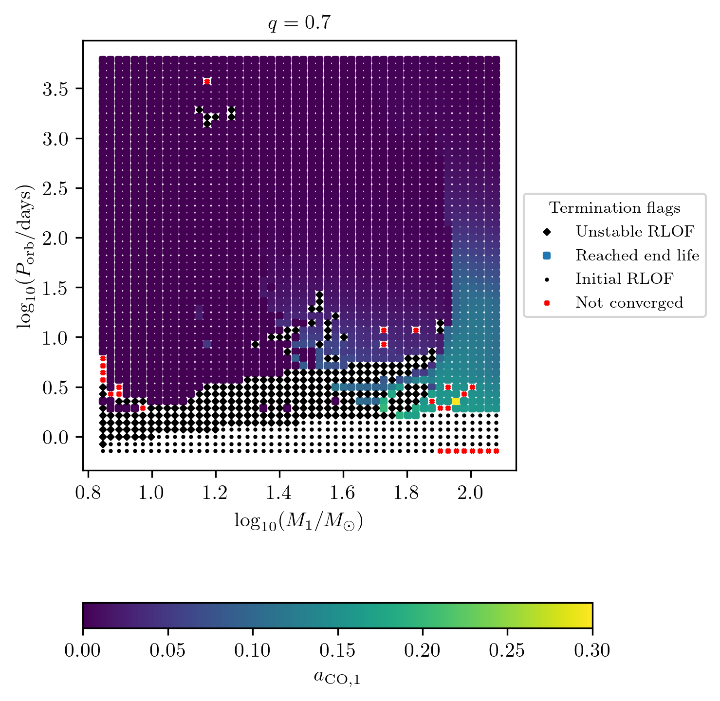
Core collapse quantities

Numerical post processed quantities can be displayed using the z variable option as shown with termination flag 1.

PLOT_PROPERTIES_CC = PLOT_PROPERTIES_TF12
PLOT_PROPERTIES_CC['fname'] = 'q_%1.1f_CC_spin.png'%q
PLOT_PROPERTIES_CC['figsize'] = (4.5,6.)
PLOT_PROPERTIES_CC['colorbar'] = {'label' : r'$a_\mathrm{CO,1}$'}
PLOT_PROPERTIES_CC['zmin'] = 0.
PLOT_PROPERTIES_CC['zmax'] = 0.3

fig = grid.plot2D('star_1_mass', 'period_days', 'S1_Patton&Sukhbold20-engineN20_spin',
             termination_flag='termination_flag_1',
             grid_3D=True, slice_3D_var_str='mass_ratio',
             slice_3D_var_range=(q-0.025,q+0.025),
             verbose=False, **PLOT_PROPERTIES_CC)

On the other hand supernova type and compact object states are stored as strings in the dataset. These quantities can be plotted using the termination_flag option of plot2D, as

PLOT_PROPERTIES_CC = PLOT_PROPERTIES_TF12
PLOT_PROPERTIES_CC['fname'] = 'q_%1.1f_CC_SN.png'%q

fig = grid.plot2D('star_1_mass', 'period_days', None,
             termination_flag='S1_Patton&Sukhbold20-engineN20_SN_type',
             grid_3D=True, slice_3D_var_str='mass_ratio',
             slice_3D_var_range=(q-0.025,q+0.025),
             verbose=False, **PLOT_PROPERTIES_CC)

PLOT_PROPERTIES_CC = PLOT_PROPERTIES_TF12
PLOT_PROPERTIES_CC['fname'] = 'q_%1.1f_CC_state.png'%q

fig = grid.plot2D('star_1_mass', 'period_days', None,
            termination_flag='S1_Patton&Sukhbold20-engineN20_state',
            grid_3D=True, slice_3D_var_str='mass_ratio',
            slice_3D_var_range=(q-0.025,q+0.025),
            verbose=False, **PLOT_PROPERTIES_CC)

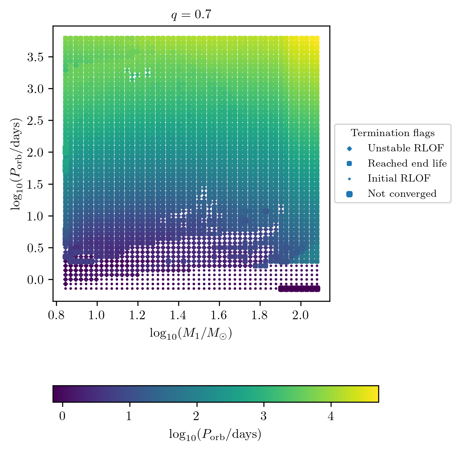
Displaying final quantities also for initial and unstable mass transfer

We have a debug termination_flag option which allows us to display as a colormap the final value also for the tracks that ends because of initial or unstable mass transfer.

PLOT_PROPERTIES_TF1 = PLOT_PROPERTIES_TF12
PLOT_PROPERTIES_TF1['fname'] = 'q_%1.1f_debug.png'%q
PLOT_PROPERTIES_TF1['figsize'] = (4.5,6.)
PLOT_PROPERTIES_TF1['log10_z'] = True

fig = grid.plot2D('star_1_mass', 'period_days', 'period_days',
             termination_flag='debug',
             grid_3D=True, slice_3D_var_str='mass_ratio',
             slice_3D_var_range=(q-0.025,q+0.025),
             verbose=False, **PLOT_PROPERTIES_TF1)

Advanced plotting options

How to plot up to onset of RLO

This functionality allows to slice the MESA runs at onset of Roche-Lobe overflow and display with a color a quantity in history1 or binary_history at onset RLO, or, alternatively one of the termination flags. Use slice_at_RLO=True option of plot2D to allow for this. Note: depending on how many runs you intend to display this might take a while.

Overplot grids

Sometimes you want to rerun a subsample of the grid. This option will allow you to stack as many grid reruns as you wish. You can combine the new grid by passing it to the option extra_grid=new_grid. If you want to stack more than one grid, pass them in a list, e.g. extra_grid=[new_grid_1,new_grid_2,new_grid_3], they will be stacked in the order provided where the last extra grid of the list will stacked as last.