1D plotting functionalities for POSYDON GRIDS
We provide a variety of 1D MESA grids plotting functions within POSYDON.
We start by loading a grid in a PSyGrid object. The plot method supports
any POSYDON MESA grid. Here, we will use the HMS-HMS grid as an example.
# to load a grid
from posydon.grids.psygrid import PSyGrid
grid = PSyGrid("/PATH_TO_POSYDON_DATA/HMS-HMS/grid_0.0142_%d.h5")
How to plot one track
Plot one quantity as a function of another
The properties to plot for a given MESA track (we have chosen the 42nd track in
the grid) can be read from history1, history2, or binary_history.
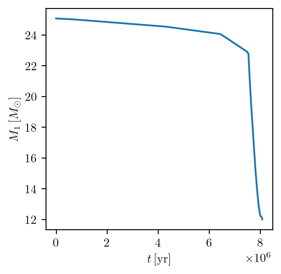
For example, to plot the mass evolution of star_1:
PLOT_PROPERTIES_1 = {
    'show_fig' : True,
    'close_fig' : True,
    'path_to_file': './plots_demo/',
    'fname': '1D_age_M1.png',
}

grid.plot(42, 'age', 'star_1_mass', history='binary_history', **PLOT_PROPERTIES_1)
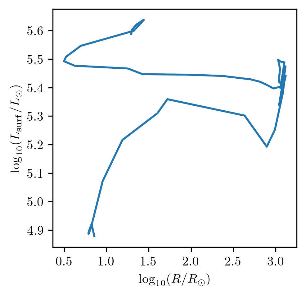
If, instead, we would like to plot the evolution of star_1 within a Hertzsprung-Russell diagram:
PLOT_PROPERTIES_2 = PLOT_PROPERTIES_1
PLOT_PROPERTIES_2['fname'] = '1D_logR_logL.png'

grid.plot(42, 'log_R', 'log_L', history='history1', **PLOT_PROPERTIES_2)
Plot multiple quantities as a function of one
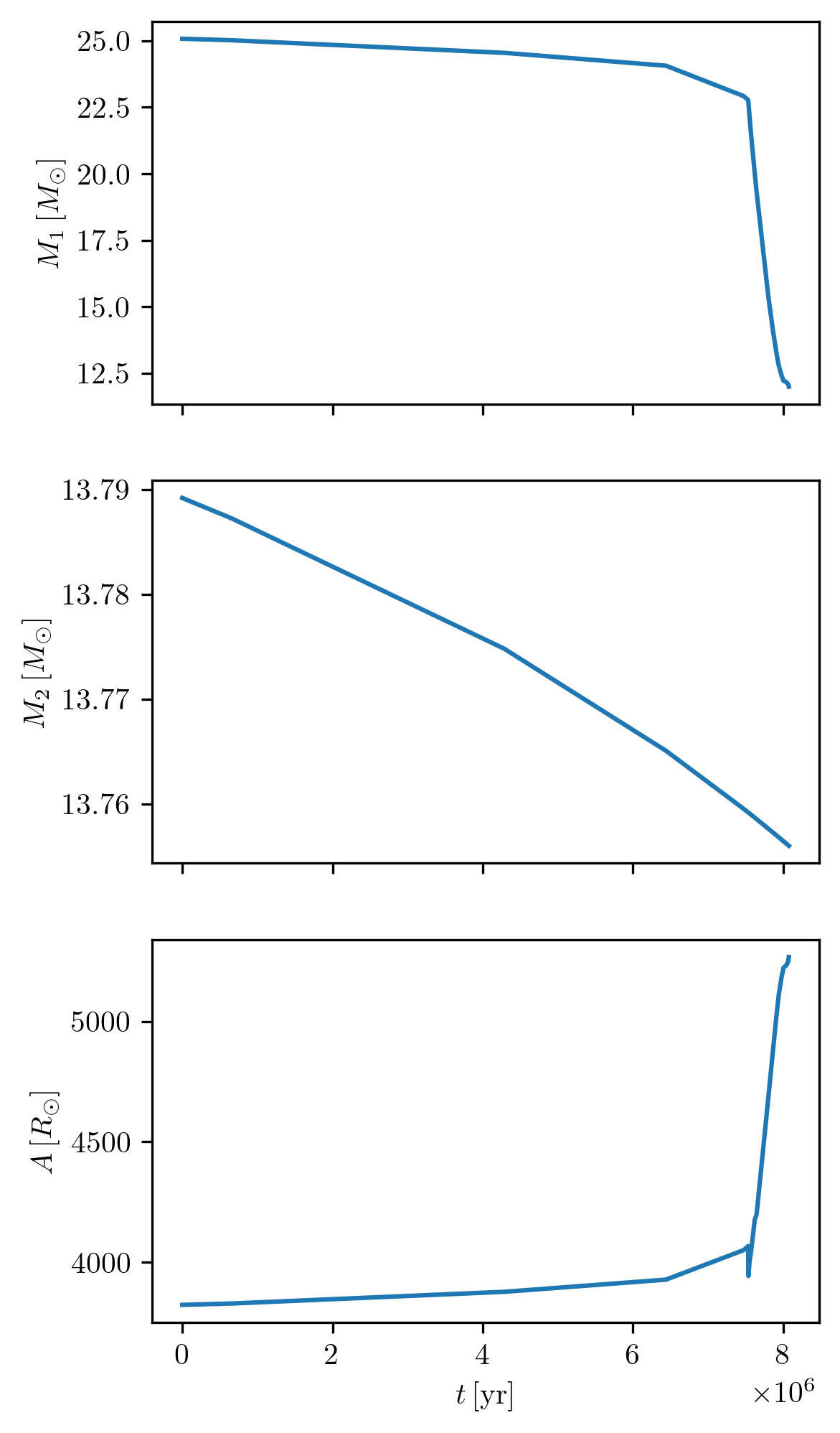
We can display more properties as a function of another in a subplot like the following examples.
PLOT_PROPERTIES_4 = PLOT_PROPERTIES_1
PLOT_PROPERTIES_4['fname'] = '1D_age_bin.png'
PLOT_PROPERTIES_4['figsize'] = (4., 8.)

grid.plot(42, 'age', ['star_1_mass', 'star_2_mass', 'binary_separation'], history='binary_history', **PLOT_PROPERTIES_4)
PLOT_PROPERTIES_3 = PLOT_PROPERTIES_1
PLOT_PROPERTIES_3['fname'] = '1D_logR_logLs.png'
PLOT_PROPERTIES_3['figsize'] = (4., 8.)

grid.plot(42, 'log_R', ['log_LH', 'log_LHe','log_LZ'], history='history1', **PLOT_PROPERTIES_3)

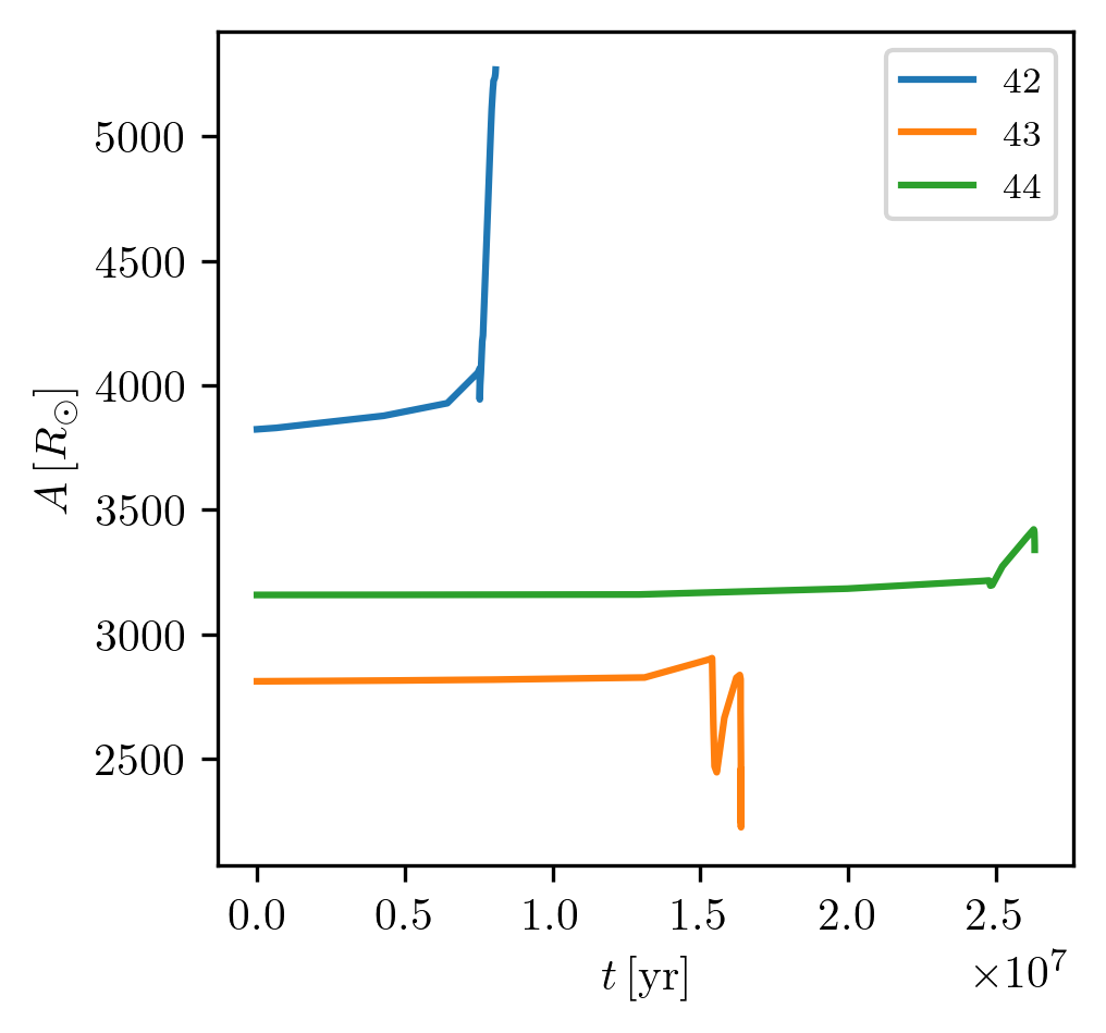
How to plot many tracks
Plot one or more quantities as a function of another for multiple tracks
If one wants to compare multiple tracks on the same plot, the indices for all binaries can be provided as a list.
PLOT_PROPERTIES_5 = PLOT_PROPERTIES_1
PLOT_PROPERTIES_5['fname'] = '1D_multi.png'
PLOT_PROPERTIES_5['legend1D'] = dict(loc='upper right', lines_legend=['42','43', '44'])

grid.plot([42,43,44], 'age', 'binary_separation', history='binary_history', **PLOT_PROPERTIES_5)
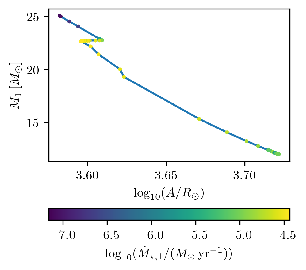
Plot third quantity as a color map
PLOT_PROPERTIES_6 = PLOT_PROPERTIES_1
PLOT_PROPERTIES_6['fname'] = '1D_color.png'
PLOT_PROPERTIES_6['log10_x'] = True

grid.plot(42, 'binary_separation', 'star_1_mass', 'lg_mstar_dot_1', history='binary_history', **PLOT_PROPERTIES_6)
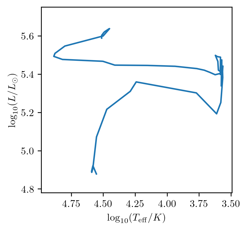
Plotting an HR diagram
One can use the HR method to display the HR diagram.
Note that multiple tracks at once can also be displayed.
PLOT_PROPERTIES_7 = PLOT_PROPERTIES_1
PLOT_PROPERTIES_7['fname'] = 'HR1.png'

grid.HR(42, history='history1', **PLOT_PROPERTIES_7)
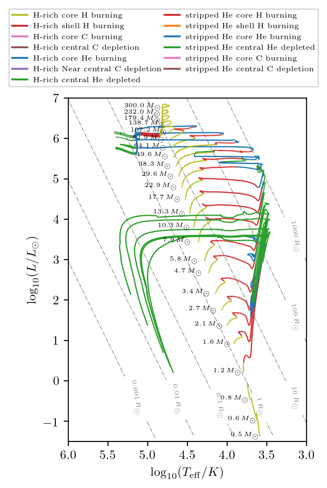
The HR diagram method has also an option to display the stellar state.
Here we show how to reproduce the HR diagram of Fig. 5 in Fragos et al. (2022).
import numpy as np

# load single HMS grid
grid = PSyGrid("/Volumes/T7/data_phd/POSYDON/data/POSYDON_data/single_HMS/grid_0.0142.h5")

PLOT_PROPERTIES_8 = {
    'figsize' : (3.38, 5),
    'show_fig' : True,
    'close_fig' : True,
    'path_to_file': './plots_demo/',
    'fname': 'HR2.png',
    'xmin' : 3.,
    'xmax' : 6.,
    'ymin' : -1.5,
    'ymax' : 7.,
    'const_R_lines' : True,
    'legend1D' : {
        'loc' : 'upper center',
        'bbox_to_anchor' : (0.4, 1.27),
        'ncol' : 2,
        'prop': {
            'size': 6
        },
        }
}

# chose a subsample of tracks
idx = np.around(np.argsort(grid.initial_values['S1_star_mass']),2)[::8]
idx = list(set(idx)-{10, 82, 128, 166})+[101,14,96,191]

grid.HR(idx, history='history1', states=True, **PLOT_PROPERTIES_8)