Explore the assumption of star-formation history and DCO compute rates at one single metallicity 📖

If you haven’t done so yet, export the path POSYDON environment variables. For example:

%env PATH_TO_POSYDON=/Users/simone/Google Drive/github/POSYDON-public/
%env PATH_TO_POSYDON_DATA=/Volumes/T7/

env: PATH_TO_POSYDON=/Users/simone/Google Drive/github/POSYDON-public/
env: PATH_TO_POSYDON_DATA=/Volumes/T7/

Creating the Synthetic Poupulation DataFrame

We will use the same BBH population as in the Analyzing Merging BBH Populations: Rates & Observations tutorial. Instead of computing the distributions and rates at all metallicities, we will just focus on one metallicity, \(Z_\odot\), and integrate the star formation history around solar metallicity, say \([0.5Z_\odot,2Z_\odot]\). Let’s extract the merging BBH population from the \(Z_\odot\) population synthesis model. In this sample there are only ~200 systems, to increase the statistics we suggest you run a population containing x50 more binaries.

import os
from posydon.popsyn.synthetic_population import SyntheticPopulation
from posydon.config import PATH_TO_POSYDON_DATA

path = os.path.join(PATH_TO_POSYDON_DATA, "POSYDON_data/tutorials/population-synthesis/example/")
files = [f for f in os.listdir(path) if '1.00e+00_Zsun_population' in f]
path_to_data = [os.path.join(path, file) for file in files]

pop = SyntheticPopulation(path_to_ini='./population_params.ini', verbose=True)

pop.parse( path_to_data=path_to_data, S1_state='BH', S2_state='BH', binary_state='contact', invert_S1S2=False)
pop.save_pop(os.path.join(path,'BBH_population_1e+00_Zsun.h5'))

pop.df.head(10)
del pop

Binary count with (S1_state, S2_state, binary_state, binary_event) equal
to (BH, BH, contact, None)
in /Volumes/T7/POSYDON_data/tutorials/population-synthesis/example/1.00e+00_Zsun_population.h5 are 233
Total binaries found are 233
Population successfully saved!

/Users/simone/Google Drive/github/POSYDON-public/posydon/popsyn/synthetic_population.py:300: PerformanceWarning:
your performance may suffer as PyTables will pickle object types that it cannot
map directly to c-types [inferred_type->mixed,key->block1_values] [items->Index(['state', 'event', 'step_names', 'S1_state', 'S2_state'], dtype='object')]

  self.df.to_hdf(path, key='history')
/Users/simone/Google Drive/github/POSYDON-public/posydon/popsyn/synthetic_population.py:301: PerformanceWarning:
your performance may suffer as PyTables will pickle object types that it cannot
map directly to c-types [inferred_type->mixed,key->block2_values] [items->Index(['state_i', 'event_i', 'step_names_i', 'state_f', 'event_f',
       'step_names_f', 'S1_state_i', 'S1_state_f', 'S1_SN_type', 'S2_state_i',
       'S2_state_f', 'S2_SN_type', 'interp_class_HMS_HMS',
       'interp_class_CO_HMS_RLO', 'interp_class_CO_HeMS',
       'interp_class_CO_HeMS_RLO', 'mt_history_HMS_HMS',
       'mt_history_CO_HMS_RLO', 'mt_history_CO_HeMS',
       'mt_history_CO_HeMS_RLO'],
      dtype='object')]

  self.df_oneline.to_hdf(path, key='oneline')

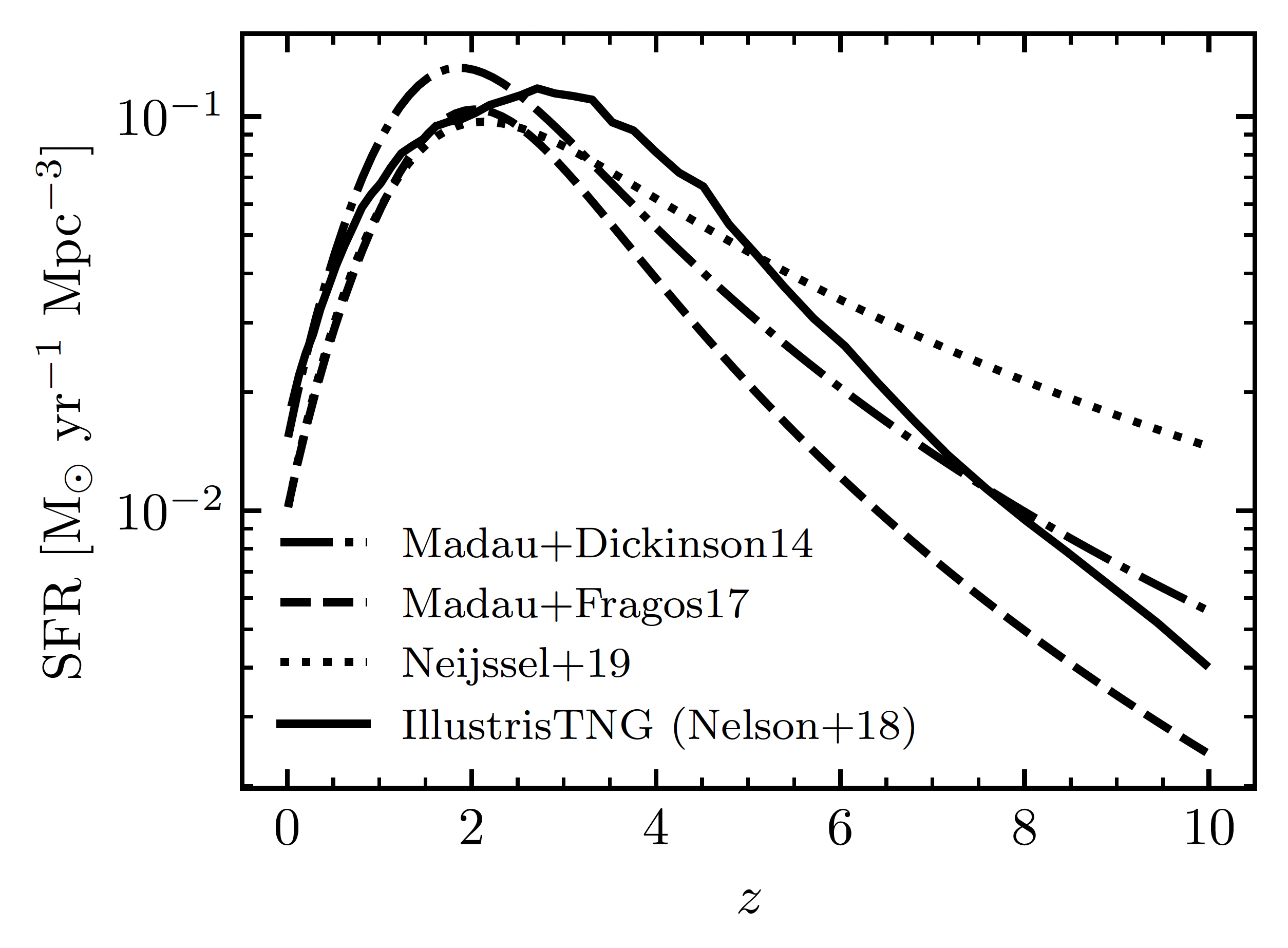
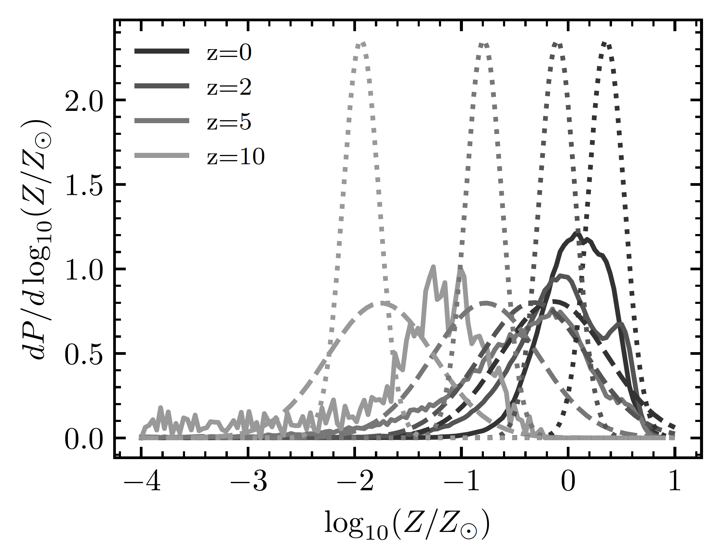
POSYDON supports different assumptions for the star formation history, e.g. instead of using the IllustrisTNG SFH, we can use the star formation rate from Madau & Fragos (2018) (see Andrews et al. in prep.) and assume a log-normal metallicity distribution around the empirically measured mean metallicity at each redshift from Madau & Fragos (2018), taking a dispersion of 0.5 dex (see Bavera et al. 2020). The IllustrisTNG star formation rate and metallicity evolution (solid line) is compared to the Madau & Fragos (2018) metallicity evolution (dashed line) in Fig. X of (see Andrews et al. in prep.), which figure is reproduced below. The dotted line corresponds to the metallicity distribution of Neijssel et al. (2019).

import os
import numpy as np
from posydon.config import PATH_TO_POSYDON_DATA
from posydon.popsyn.synthetic_population import SyntheticPopulation

# cosmological model parameters for the rate calculation
MODEL = {
    'delta_t' : 100, # Myr
    'SFR' : 'Madau+Fragos17',
    'sigma_SFR' : 'Bavera+20',
    'Z_max' : 1.,
    'Zsun' : 0.0142,
    'select_one_met' : True,
    'dlogZ' : [np.log10(0.0142/2),np.log10(0.0142*2)],
}

pop = SyntheticPopulation('./population_params.ini', verbose=True, MODEL=MODEL)
path = os.path.join(PATH_TO_POSYDON_DATA, "POSYDON_data/tutorials/population-synthesis/example/")
pop.load_pop(os.path.join(path,'BBH_population_1e+00_Zsun.h5'))

# generate the BBH synthetic population
pop.get_dco_at_formation(S1_state='BH', S2_state='BH',
                         oneline_cols=['S1_natal_kick_array_0', 'S2_natal_kick_array_0'],
                         formation_channels=True)

# we can save the synthetic population
# pop.save_synthetic_pop(os.path.join(path,'BBH_synthetic_population.h5'))
# pop.load_synthetic_pop(os.path.join(path,'BBH_synthetic_population.h5'))

cols = ['metallicity','time','t_delay','S1_state','S2_state','S1_mass','S2_mass',
        'S1_spin','S2_spin', 'orbital_period','eccentricity', 'channel']
pop.df_synthetic[cols]

Population successfully loaded!
Computing formation channels...

/Users/simone/Google Drive/github/POSYDON-public/posydon/popsyn/synthetic_population.py:804: FutureWarning: Setting an item of incompatible dtype is deprecated and will raise in a future error of pandas. Value 'ZAMS_oDoubleCE1_CC1_redirect_CC2_CO_contact_END' has dtype incompatible with float64, please explicitly cast to a compatible dtype first.
  self.df_oneline.loc[index,'channel_debug'] = formation_channel
/Users/simone/Google Drive/github/POSYDON-public/posydon/popsyn/synthetic_population.py:808: FutureWarning: Setting an item of incompatible dtype is deprecated and will raise in a future error of pandas. Value 'ZAMS_oDoubleCE1_CC1_CC2_END' has dtype incompatible with float64, please explicitly cast to a compatible dtype first.
  self.df_oneline.loc[index,'channel'] = formation_channel

	metallicity	time	t_delay	S1_state	S2_state	S1_mass	S2_mass	S1_spin	S2_spin	orbital_period	eccentricity	channel
0	0.0142	4.027170	2913.863804	BH	BH	13.120462	12.911080	0.079649	0.064849	1.611464	0.048133	ZAMS_oDoubleCE1_CC1_CC2_END
1	0.0142	4.027170	1500.583774	BH	BH	13.120462	12.911080	0.079649	0.063991	1.279098	0.123592	ZAMS_oDoubleCE1_CC1_CC2_END
2	0.0142	4.849573	662.821800	BH	BH	10.330899	9.888130	0.286911	0.249267	0.817643	0.165775	ZAMS_oDoubleCE1_CC1_CC2_END
3	0.0142	4.544886	845.424610	BH	BH	11.355246	10.251920	0.320931	0.298164	1.108194	0.379450	ZAMS_oDoubleCE1_CC1_CC2_END
4	0.0142	4.530889	620.499837	BH	BH	11.436823	10.900538	0.190982	0.167996	0.830194	0.107165	ZAMS_oDoubleCE1_CC1_CC2_END
...	...	...	...	...	...	...	...	...	...	...	...	...
228	0.0142	7.928745	426.765027	BH	BH	17.564588	8.155695	0.040933	0.015301	17.694336	0.957889	ZAMS_oRLO1_CC1_oRLO2_CC2_END
229	0.0142	4.530889	787.032676	BH	BH	11.436823	10.900538	0.190982	0.168671	0.894027	0.022964	ZAMS_oDoubleCE1_CC1_CC2_END
230	0.0142	4.848528	943.501358	BH	BH	10.331316	9.972710	0.312185	0.277781	0.911809	0.093335	ZAMS_oDoubleCE1_CC1_CC2_END
231	0.0142	4.256912	1266.769326	BH	BH	12.239574	11.551092	0.179405	0.165071	1.159215	0.175475	ZAMS_oDoubleCE1_CC1_CC2_END
232	0.0142	4.537286	658.997955	BH	BH	11.338870	10.753148	0.269757	0.242801	0.851837	0.137036	ZAMS_oDoubleCE1_CC1_CC2_END

233 rows × 12 columns

Compute the BBH Merger Rates for \(Z\in [0.5Z_\odot,2Z_\odot]\)

Similar to the Analyzing Merging BBH Populations: Rates & Observations we compute the BBH merger rate density to obtain the BBH intrinsic population.

pop.get_dco_merger_rate_density()
# pop.save_intrinsic_pop(os.path.join(path,'BBH_intrinsic_population.h5'))
# pop.load_intrinsic_pop(os.path.join(path,'BBH_intrinsic_population.h5'))
pop.df_dco_intrinsic[cols]

100%|██████████| 138/138 [00:00<00:00, 162.70it/s]
100%|██████████| 7/7 [00:09<00:00,  1.30s/it]

DCO merger rate density in the local Universe (z=0.00): 10.74 Gpc^-3 yr^-1

	metallicity	time	t_delay	S1_state	S2_state	S1_mass	S2_mass	S1_spin	S2_spin	orbital_period	eccentricity	channel
0	0.0142	6.205715	4.287125e-08	BH	BH	12.260188	12.183039	0.050168	8.244612e-04	326.580311	0.999994	ZAMS_CC1_oRLO2_CC2_END
1	0.0142	4.705799	9.754266e-01	BH	BH	12.850735	20.143346	0.027546	5.791334e-17	2377.230212	0.999817	ZAMS_CC1_CC2_END
2	0.0142	8.187239	2.075700e+00	BH	BH	8.314851	8.315119	0.100591	6.554160e-03	38.651550	0.996045	ZAMS_oRLO1-reverse_CC1_CC2_END
3	0.0142	6.647572	2.472628e+01	BH	BH	9.826765	9.853595	0.032525	2.400078e-02	14.240625	0.980550	ZAMS_oRLO1-contact_CC1_CC2_END
4	0.0142	6.676527	1.680554e+01	BH	BH	20.974131	12.500642	0.000531	4.772162e-04	696.487802	0.998932	ZAMS_CC1_oRLO2_CC2_END
...	...	...	...	...	...	...	...	...	...	...	...	...
26870	0.0142	7.928745	4.267650e+02	BH	BH	17.564588	8.155695	0.040933	1.530132e-02	17.694336	0.957889	ZAMS_oRLO1_CC1_oRLO2_CC2_END
26871	0.0142	4.530889	7.870327e+02	BH	BH	11.436823	10.900538	0.190982	1.686708e-01	0.894027	0.022964	ZAMS_oDoubleCE1_CC1_CC2_END
26872	0.0142	4.848528	9.435014e+02	BH	BH	10.331316	9.972710	0.312185	2.777810e-01	0.911809	0.093335	ZAMS_oDoubleCE1_CC1_CC2_END
26873	0.0142	4.256912	1.266769e+03	BH	BH	12.239574	11.551092	0.179405	1.650709e-01	1.159215	0.175475	ZAMS_oDoubleCE1_CC1_CC2_END
26874	0.0142	4.537286	6.589980e+02	BH	BH	11.338870	10.753148	0.269757	2.428005e-01	0.851837	0.137036	ZAMS_oDoubleCE1_CC1_CC2_END

26875 rows × 12 columns

pop.plot_rate_density(DCO=True, channels=True, **{'ylim' : [0.01, 100]})

pop.get_dco_detection_rate(sensitivity='design_H1L1V1') # if already computed use load_data=True
# pop.save_observable_pop(os.path.join(path,'BBH_observable_population.h5'))
# pop.load_observable_pop(os.path.join(path,'BBH_observable_population.h5'))
pop.df_dco_observable[cols]

100%|██████████| 138/138 [00:13<00:00, 10.45it/s]

DCO detection rate at design_H1L1V1 sensitivity: 590.18 yr^-1

	metallicity	time	t_delay	S1_state	S2_state	S1_mass	S2_mass	S1_spin	S2_spin	orbital_period	eccentricity	channel
0	0.0142	6.205715	4.287125e-08	BH	BH	12.260188	12.183039	0.050168	8.244612e-04	326.580311	0.999994	ZAMS_CC1_oRLO2_CC2_END
1	0.0142	4.705799	9.754266e-01	BH	BH	12.850735	20.143346	0.027546	5.791334e-17	2377.230212	0.999817	ZAMS_CC1_CC2_END
2	0.0142	8.187239	2.075700e+00	BH	BH	8.314851	8.315119	0.100591	6.554160e-03	38.651550	0.996045	ZAMS_oRLO1-reverse_CC1_CC2_END
3	0.0142	6.647572	2.472628e+01	BH	BH	9.826765	9.853595	0.032525	2.400078e-02	14.240625	0.980550	ZAMS_oRLO1-contact_CC1_CC2_END
4	0.0142	6.676527	1.680554e+01	BH	BH	20.974131	12.500642	0.000531	4.772162e-04	696.487802	0.998932	ZAMS_CC1_oRLO2_CC2_END
...	...	...	...	...	...	...	...	...	...	...	...	...
19536	0.0142	7.214096	1.052488e+04	BH	BH	12.340761	8.201690	0.185531	1.411149e-01	2.783007	0.396922	ZAMS_CC1_oRLO2_CC2_END
19537	0.0142	3.443633	6.236191e+03	BH	BH	12.585380	12.508058	0.090103	2.004811e-03	250.806290	0.988294	ZAMS_CC1_CC2_END
19538	0.0142	4.900714	4.178555e+03	BH	BH	17.470438	16.106886	0.202329	4.508136e-04	1580.389855	0.997143	ZAMS_oRLO1-reverse_CC1_CC2_END
19539	0.0142	7.154675	8.766378e+03	BH	BH	10.272165	9.248458	0.090886	1.197166e-01	3.129920	0.527011	ZAMS_oRLO1_CC1_oRLO2_CC2_END
19540	0.0142	3.781907	7.804838e+03	BH	BH	10.729561	11.898371	0.179142	6.654702e-02	81.451235	0.971019	ZAMS_CC1_CC2_END

19541 rows × 12 columns

Visaulize the BBH Population Properties

kwargs = dict(bins=50, xlog=False)
pop.plot_hist_properties('m_chirp', intrinsic=True, observable=True, pop='DCO', **kwargs)
pop.plot_hist_properties('chi_eff', intrinsic=True, observable=True, pop='DCO', **kwargs)
pop.plot_hist_properties(['S1_mass','S2_mass'], intrinsic=True, observable=True, pop='DCO', **kwargs)
pop.plot_hist_properties(['S1_spin','S2_spin'], intrinsic=True, observable=True, pop='DCO', **kwargs)