2D Plotting Functionalities for POSYDON PSyGrids
This tutorial shows you how to plot single and binary stellar tracks using the plot2D visualization library. The plot2D method supports either a MESA grid which samples the 2D parameter space of binary initial conditions in a 2D, 3D or 4D MESA space, e.g., star_1_mass, star_2_mass (or mass ratio), period_days, metallicity. In the 3D and 4D cases the MESA grid will be sliced along the dimensions specified by the user.
If you haven’t done it already, export the environemnt variables.
[1]:
%env PATH_TO_POSYDON=/Users/simone/Google Drive/github/POSYDON-public/
%env PATH_TO_POSYDON_DATA=/Volumes/T7/
env: PATH_TO_POSYDON=/Users/simone/Google Drive/github/POSYDON-public/
env: PATH_TO_POSYDON_DATA=/Volumes/T7/
Any plotting parameter is passed to the plot2D method through the kwarg PLOT_PROPERTIES. Note that you can save each plot to a given path_to_file by specifying the filename `fname.
Example: the HMS-HMS gird
Let’s start by loading the grid.
[2]:
import os
from posydon.config import PATH_TO_POSYDON_DATA
from posydon.grids.psygrid import PSyGrid

path_to_gird = os.path.join(PATH_TO_POSYDON_DATA, 'POSYDON_data/HMS-HMS/1e-01_Zsun.h5')
grid = PSyGrid(path_to_gird)
grid.load()
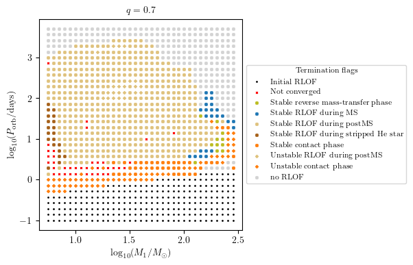
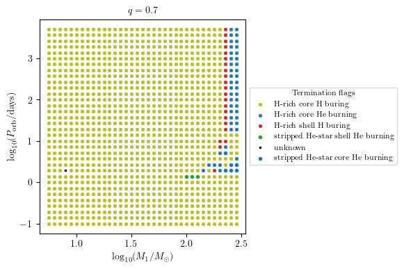
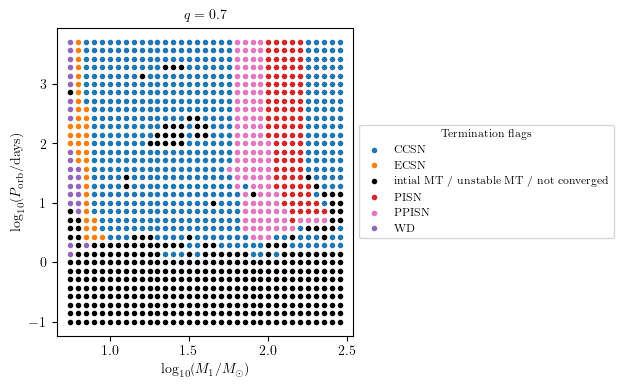
MESA Termination Flags 1 and 2 Combied
This plot summarise the binary evolutioary simulation.
[7]:
q = 0.7
PLOT_PROPERTIES = {
    'figsize': (4.5, 4.),
    'show_fig' : True,
    'close_fig' : True,
    #'path_to_file': './dirname/',
    #'fname': f'filename_q_{q}.png', # specify the filename if you want to save the figure
    'title' : r'$q = %1.1f$'%q,
    'log10_x' : True,
    'log10_y' : True,
}

grid.plot2D('star_1_mass', 'period_days', None,
            termination_flag='combined_TF12',
            grid_3D=True, slice_3D_var_str='mass_ratio',
            slice_3D_var_range=(q-0.025,q+0.025),
            verbose=False, **PLOT_PROPERTIES)
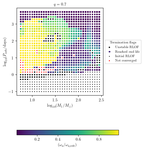
MESA Termination Flag 1
This plot indicates why MESA stopped and allows to illustrata a final quantity.
[10]:
PLOT_PROPERTIES['figsize'] = (4.5,6.)

grid.plot2D('star_1_mass', 'period_days', 'S2_surf_avg_omega_div_omega_crit',
            termination_flag='termination_flag_1',
            grid_3D=True, slice_3D_var_str='mass_ratio',
            slice_3D_var_range=(q-0.025,q+0.025),
            verbose=False, **PLOT_PROPERTIES)
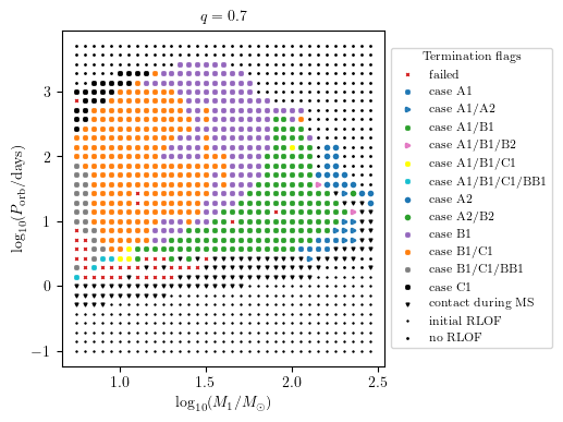
MESA Termination Flag 2
The termination flag 2 shows a summary of all mass transfer cases which occurred during the binaries’ evolution.
[12]:
PLOT_PROPERTIES['figsize'] = (4.5,4.) # defualt

grid.plot2D('star_1_mass', 'period_days', None,
            termination_flag='termination_flag_2',
            grid_3D=True, slice_3D_var_str='mass_ratio',
            slice_3D_var_range=(q-0.025,q+0.025),
            verbose=False, **PLOT_PROPERTIES)
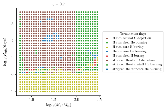
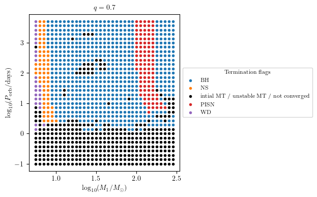
MESA Termination Flag 3 and 4
The termination flag 3/ shows the final stellar state of star 1/2.
[13]:
grid.plot2D('star_1_mass', 'period_days', None,
            termination_flag='termination_flag_3',
            grid_3D=True, slice_3D_var_str='mass_ratio',
            slice_3D_var_range=(q-0.025,q+0.025),
            verbose=False, **PLOT_PROPERTIES)
[8]:
grid.plot2D('star_1_mass', 'period_days', None,
            termination_flag='termination_flag_4',
            grid_3D=True, slice_3D_var_str='mass_ratio',
            slice_3D_var_range=(q-0.025,q+0.025),
            verbose=False, **PLOT_PROPERTIES)
One can plot all termination flags at once in a large subplot of panels with the option termination_flag='all'. In order to fit all legends we suggest to increase the figure size and marker size to, e.g. (25,25) and 30, respectively.
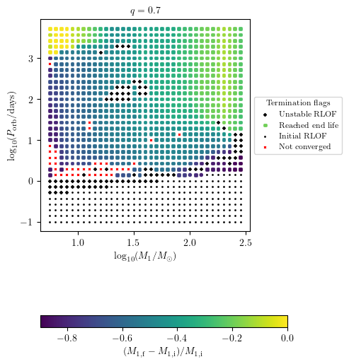
Display Relative Change of a Final Quantity
The relative change of any value stored within final_values can be displayed by adding the prefix relative_change_ to the z-variable displayed as a colorbar. E.g. we can display the relative change of star_1_mass:
[12]:
PLOT_PROPERTIES['figsize'] = (4.5,6.)
PLOT_PROPERTIES['colorbar'] = {'label' : r'$(M_\mathrm{1,f}-M_\mathrm{1,i})/M_\mathrm{1,i}$',}

grid.plot2D('star_1_mass', 'period_days', 'relative_change_star_1_mass',
            termination_flag='termination_flag_1',
            grid_3D=True, slice_3D_var_str='mass_ratio',
            slice_3D_var_range=(q-0.025,q+0.025),
            verbose=False, **PLOT_PROPERTIES)
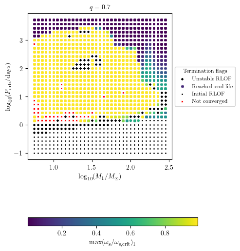
Display Custom Quantities
The user can plot custom quantities as a color map on termination flag 1. For example, we display the maximum surf_avg_omega_div_omega_crit during the history of star 2 as follows
[14]:
import numpy as np
PLOT_PROPERTIES['figsize'] = (4.5,6.)
PLOT_PROPERTIES['colorbar'] = {'label' : r'$\max(\omega_\mathrm{s}/\omega_\mathrm{s,crit})_1$'}

max_omega = [max(grid[i].history2['surf_avg_omega_div_omega_crit'])
            if grid[i].history2 is not None else np.nan
            for i in range(len(grid.MESA_dirs))]

grid.plot2D('star_1_mass', 'period_days', np.array(max_omega),
            termination_flag='termination_flag_1',
            grid_3D=True, slice_3D_var_str='mass_ratio',
            slice_3D_var_range=(q-0.025,q+0.025),
            verbose=False, **PLOT_PROPERTIES)
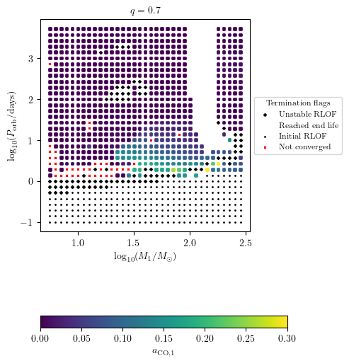
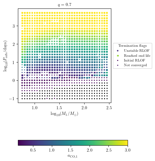
Dispaly Core Collapse Quantities
Float quantities can be displayed using the z variable option as shown with termination flag 1.
[16]:
PLOT_PROPERTIES['figsize'] = (4.5,6.)
PLOT_PROPERTIES['colorbar'] = {'label' : r'$a_\mathrm{CO,1}$'}
PLOT_PROPERTIES['zmin'] = 0.
PLOT_PROPERTIES['zmax'] = 0.3

grid.plot2D('star_1_mass', 'period_days', 'S1_MODEL05_spin',
            termination_flag='termination_flag_1',
            grid_3D=True, slice_3D_var_str='mass_ratio',
            slice_3D_var_range=(q-0.025,q+0.025),
            verbose=False, **PLOT_PROPERTIES)
[ ]:
The missig points in the above plots are NaN values associated to disruped stars due to pair instability supernovae (PISN).

To display supernova type (SN_type) and compact object type (CO_type) are stored as strings in the dataset. These quantities can be plotted using the ``termination_flag`` option of ``plot2D``, as
[17]:
PLOT_PROPERTIES['figsize'] = (4.5,4.) # defualt

grid.plot2D('star_1_mass', 'period_days', None,
               termination_flag='S1_MODEL01_SN_type',
               grid_3D=True, slice_3D_var_str='mass_ratio',
               slice_3D_var_range=(q-0.025,q+0.025),
               verbose=False, **PLOT_PROPERTIES)

grid.plot2D('star_1_mass', 'period_days', None,
               termination_flag='S1_MODEL01_CO_type',
               grid_3D=True, slice_3D_var_str='mass_ratio',
               slice_3D_var_range=(q-0.025,q+0.025),
               verbose=False, **PLOT_PROPERTIES)
Displaying Final Quantities also for intial_MT, unstable_MT and not_converged Interpolationn Classes
We have a debug termination_flag option which allows us to display as a colormap the final value also for the tracks that ends because of initial or unstable mass transfer.
[20]:
PLOT_PROPERTIES['figsize'] = (4.5,6.)
PLOT_PROPERTIES['log10_z'] = True
PLOT_PROPERTIES['zmin'] = 0.1
PLOT_PROPERTIES['zmax'] = 3

grid.plot2D('star_1_mass', 'period_days', 'period_days',
            termination_flag='debug',
            grid_3D=True, slice_3D_var_str='mass_ratio',
            slice_3D_var_range=(q-0.025,q+0.025),
            verbose=False, **PLOT_PROPERTIES)
Advanced Plotting Functionalities
How to plot grid up to onset of RLO
This functionality allows to slice the MESA runs at onset of Roche-Lobe overflow and display with a color a quantity in history1 or binary_history at onset RLO, or, alternatively one of the termination flags. Use slice_at_RLO=True option of plot2D to allow for this. Note: depending on how many runs you intend to display this might take a while.
Overplot grids on top of each others
Sometimes you want to rerun a subsample of the grid. This option will allow you to stack as many grid reruns as you wish. You can combine the new grid by passing it to the option extra_grid=new_grid. If you want to stack more than one grid, pass them in a list, e.g. extra_grid=[new_grid_1,new_grid_2,new_grid_3], they will be stacked in the order provided where the last extra grid of the list will stacked as last.
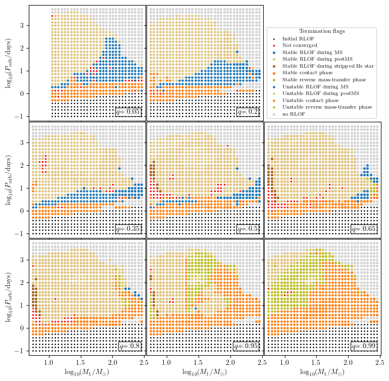
Creating plots with several slices
We have the option to pass a list of slice ranges. In this case the plotting script will loop over those ranges and create one plot with several slice plots. It will get a common legend and/or color bar.
There are two more options to the plot2D function:
max_cols: It specifies the maximum number of columns of subplots. The number of rows is automatically calculated to cover all plots and the legend.legend_pos: It specifies which subplots are used for the legend/color bar and allows an index or tuple specifying a rectangle of indecies, like matplotlib requires for creating a subplot.
Because the legend has its own axes, it is recommended to modify the default bbox_to_anchor of the legend. To have a better control on the color bar, it got the additional field bounds in the plot properties. To identify the subplots each of them will get a text box. Its attributes can be modified by changing the field slice_text_kwargs in the plot properties. The slices will loop over 3D and 4D idependently. If one of them has just a single range, this slicing will be added to the
legend title instead of being reported in any subplot.
[26]:
q_ranges = [(0.025, 0.075), (0.175, 0.225), (0.325, 0.375), (0.475, 0.525),
            (0.625, 0.675), (0.775, 0.825), (0.925, 0.975), (0.98, 1.0)]

plot_properties = {
    'show_fig': True,
    'figsize': (9, 9),
    'log10_x': True,
    'log10_y': True,
    'xmin': 0.68,
    'xmax': 2.52,
    'ymin': -1.2,
    'ymax': 3.9,
    'wspace': 0.01,
    'hspace': 0.01,
    'colorbar': {
        'bounds': [0.03, 0.7, 0.94, 0.05]
    },
    'legend2D': {
        'title': 'Termination flags',
        'loc': 'lower left',
        'prop': {
            'size': 7
        },
        'bbox_to_anchor': (0.0, 0.0),
    },
}
grid.plot2D('star_1_mass', 'period_days', None,
            termination_flag='combined_TF12',
            grid_3D=True, slice_3D_var_str='mass_ratio',
            slice_3D_var_range=q_ranges,
            legend_pos = (3,3),
            verbose=False, **plot_properties)
Creating plots with several slices at different metallicities
TODO: add the plot
Congratulations! You are now a POSYDON PSyGrid visualization expert!
[ ]: