1D Plotting Functionalities for POSYDON PSyGrids

This tutorial shows you how to plot single and binary stellar tracks using the plot1D visualization library. If you haven’t done it already, export the environemnt variables.

%env PATH_TO_POSYDON=/Users/simone/Google Drive/github/POSYDON-public/
%env PATH_TO_POSYDON_DATA=/Volumes/T7/

env: PATH_TO_POSYDON=/Users/simone/Google Drive/github/POSYDON-public/
env: PATH_TO_POSYDON_DATA=/Volumes/T7/

Example: the HMS-HMS gird

Let’s start by loading the grid.

import os
from posydon.config import PATH_TO_POSYDON_DATA
from posydon.grids.psygrid import PSyGrid

path_to_gird = os.path.join(PATH_TO_POSYDON_DATA, 'POSYDON_data/HMS-HMS/1e-01_Zsun.h5')
grid = PSyGrid(path_to_gird)
grid.load()

Plot one quantity as a function of another

We arbitrary choose the binary 42 to illustrate the plotting funtionalities. You can plot quantities stored in: history1, history2, or binary_history.

import numpy as np
print('binary_history columns:', np.squeeze(grid[42].binary_history.dtype.names))
print('')
print('history1/2 columns:', np.squeeze(grid[42].history1.dtype.names))

binary_history columns: ['model_number' 'age' 'star_1_mass' 'star_2_mass' 'period_days'
 'binary_separation' 'lg_system_mdot_1' 'lg_system_mdot_2'
 'lg_wind_mdot_1' 'lg_wind_mdot_2' 'lg_mstar_dot_1' 'lg_mstar_dot_2'
 'lg_mtransfer_rate' 'xfer_fraction' 'rl_relative_overflow_1'
 'rl_relative_overflow_2' 'trap_radius' 'acc_radius' 't_sync_rad_1'
 't_sync_conv_1' 't_sync_rad_2' 't_sync_conv_2']

history1/2 columns: ['he_core_mass' 'c_core_mass' 'o_core_mass' 'he_core_radius'
 'c_core_radius' 'o_core_radius' 'center_h1' 'center_he4' 'center_c12'
 'center_n14' 'center_o16' 'surface_h1' 'surface_he4' 'surface_c12'
 'surface_n14' 'surface_o16' 'c12_c12' 'center_gamma' 'avg_c_in_c_core'
 'surf_avg_omega' 'surf_avg_omega_div_omega_crit' 'log_LH' 'log_LHe'
 'log_LZ' 'log_Lnuc' 'log_Teff' 'log_L' 'log_R' 'log_center_T'
 'log_center_Rho' 'total_moment_of_inertia' 'spin_parameter'
 'log_total_angular_momentum' 'conv_env_top_mass' 'conv_env_bot_mass'
 'conv_env_top_radius' 'conv_env_bot_radius' 'conv_env_turnover_time_g'
 'conv_env_turnover_time_l_b' 'conv_env_turnover_time_l_t'
 'envelope_binding_energy' 'mass_conv_reg_fortides'
 'thickness_conv_reg_fortides' 'radius_conv_reg_fortides'
 'lambda_CE_1cent' 'lambda_CE_10cent' 'lambda_CE_30cent' 'co_core_mass'
 'co_core_radius' 'lambda_CE_pure_He_star_10cent' 'log_L_div_Ledd']

PLOT_PROPERTIES = {
    'show_fig' : True,
    'close_fig' : True,
    #'path_to_file': './dirname/',
    #'fname': 'filename.png', # specify the file name if you want to safe the figure
}

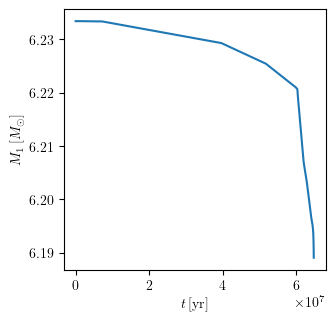
grid.plot(42, 'age', 'star_1_mass', history='binary_history', **PLOT_PROPERTIES)
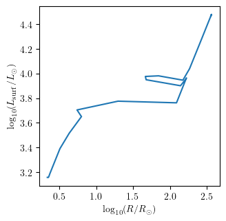
grid.plot(42,  'log_R', 'log_L', history='history1', **PLOT_PROPERTIES)

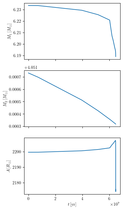
Plot multiple quantities as a function of one quantity

We can display more properties as a function of another in a subplot like the following examples.

PLOT_PROPERTIES['figsize'] = (4., 8.)

grid.plot(42, 'age', ['star_1_mass', 'star_2_mass', 'binary_separation'], history='binary_history', **PLOT_PROPERTIES)
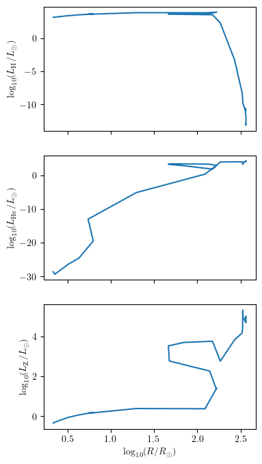
grid.plot(42, 'log_R', ['log_LH', 'log_LHe','log_LZ'], history='history1', **PLOT_PROPERTIES)

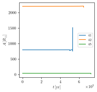
Plot one or more quantities as a function of another for multiple tracks

If one wants to compare multiple tracks on the same plot, the indices for all binaries can be provided as a list.

PLOT_PROPERTIES['figsize'] = (3.38, 3.38) # default
PLOT_PROPERTIES['legend1D'] = dict(loc='center right', lines_legend=['41','42','45'])

grid.plot([41,42,45], 'age', 'binary_separation', history='binary_history', **PLOT_PROPERTIES)

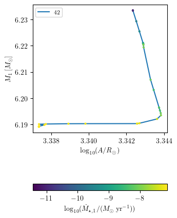
Plot a third quantity as a color map

PLOT_PROPERTIES['figsize'] = (3.38, 5)
PLOT_PROPERTIES['log10_x'] = True
PLOT_PROPERTIES['legend1D'] = dict(loc='upper left', lines_legend=['42'])

grid.plot(42, 'binary_separation', 'star_1_mass', 'lg_mstar_dot_1', history='binary_history', **PLOT_PROPERTIES)

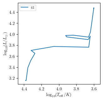
Plotting an Hertzsprung–Russell diagram

One can easily plot the Hertzsprung–Russell (HR) diagram using the HR method.

PLOT_PROPERTIES['figsize'] = (3.38, 3.38) # default

grid.HR(42, history='history1', **PLOT_PROPERTIES)

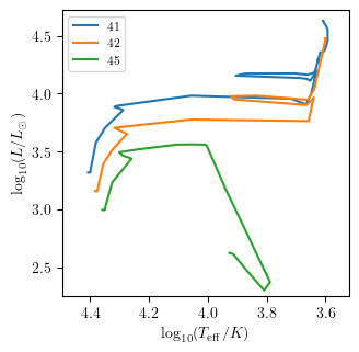
Notice that multiple tracks at once can also be displayed.

PLOT_PROPERTIES['legend1D'] = dict(loc='upper left', lines_legend=['41','42','45'])
grid.HR([41,42,45], history='history1', **PLOT_PROPERTIES)

Example: the single HMS gird

Plotting an Hertzsprung–Russell diagram

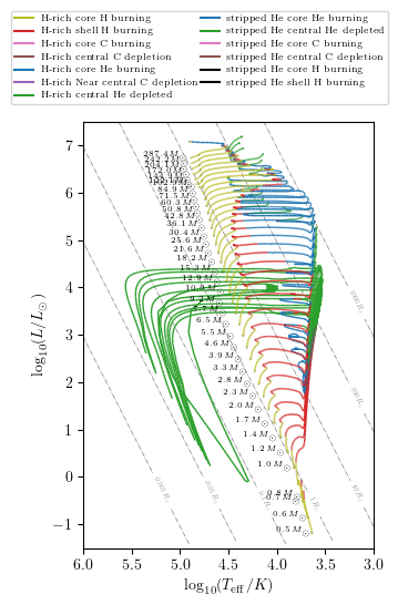
The HR diagram method has also an option to display the stellar states of the tracks. Here we show how to reproduce a HR diagram that looks like Fig. 5 in Fragos et al. (2023).

# load single HMS grid
path_to_gird = os.path.join(PATH_TO_POSYDON_DATA, 'POSYDON_data/single_HMS/1e-01_Zsun.h5')
grid = PSyGrid(path_to_gird)
grid.load()

PLOT_PROPERTIES = {
    'figsize' : (3.38, 5),
    'show_fig' : True,
    'close_fig' : True,
    #'path_to_file': './dir/',
    #'fname': 'filename.png', # specify filename to save the figure
    'xmin' : 3.,
    'xmax' : 6.,
    'ymin' : -1.5,
    'ymax' : 7.5,
    'const_R_lines' : True,
    'legend1D' : {
        'loc' : 'upper center',
        'bbox_to_anchor' : (0.4, 1.27),
        'ncol' : 2,
        'prop': {
            'size': 6
        },
        }
}

# chose a subsample of tracks
idx = np.around(np.argsort(grid.initial_values['S1_star_mass']),2)[::8].tolist()

grid.HR(idx, history='history1', states=True, **PLOT_PROPERTIES)

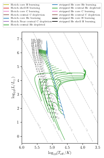
Example: the single HeMS gird

Plotting an Hertzsprung–Russell diagram

# load single HeMS grid
path_to_gird = os.path.join(PATH_TO_POSYDON_DATA, 'POSYDON_data/single_HeMS/1e-01_Zsun.h5')
grid = PSyGrid(path_to_gird)
grid.load()

PLOT_PROPERTIES['ymin'] = -0.5
PLOT_PROPERTIES['xmin'] = 3.5

# chose a subsample of tracks
idx = np.around(np.argsort(grid.initial_values['S1_star_mass']),2)[::8].tolist()

grid.HR(idx, history='history1', states=True, **PLOT_PROPERTIES)

Congratulations! You have successfully completed this tutorial. You now master POSYDON 1D visualization tools.